Note
Click here to download the full example code
Finding number of clusters
A two step PipeGraph is built by embedding a clustering algorithm such as Kmeans followed by a supervised classification algorithm such as Linear Discriminant Analysis. This kind of structure is useful in those scenarios in which the dataset comprises different subpopulations but the class labels are unknown. A common question that arises in such scenario is related to the best number of clusters. For answering that question, we might want to measure the quality of the clustering in accordance to the later capability of reproducing the results obtained by the clustering algorithm on a model based classification technique such as linear discriminant analysis.
Such PipeGraph is fit using a GridSearchCV strategy and an artificial dataset.
#%%
import matplotlib.pyplot as plt
import numpy as np
from pipegraph import PipeGraph
from sklearn import datasets
from sklearn.cluster import KMeans
from sklearn.discriminant_analysis import LinearDiscriminantAnalysis
from sklearn.metrics import confusion_matrix
from sklearn.model_selection import GridSearchCV
import seaborn as sns; sns.set()

X, y = datasets.make_blobs(n_samples=10000, n_features=5, centers=10)

clustering = KMeans(n_clusters=10)
# The values of the parameters in the initialization do not affect the grid search.

classification = LinearDiscriminantAnalysis()

steps = [('clustering', clustering),
         ('classification', classification)
         ]

model = PipeGraph(steps=steps)
model.inject(sink='clustering',     sink_var='X', source='_External',  source_var='X')
model.inject(sink='classification', sink_var='X', source='_External',  source_var='X')
model.inject(sink='classification', sink_var='y', source='clustering', source_var='predict')

n_folds = 5
number_of_clusters_to_explore = np.arange(2, 20)
search = GridSearchCV(model, param_grid=dict(clustering__n_clusters=number_of_clusters_to_explore), cv=n_folds)
search.fit(X)
#%%
The results show the CV scores along with a fill area pointing out the standard deviation bands.
# Code inspired by http://scikit-learn.org/stable/auto_examples/exercises/plot_cv_diabetes.html#sphx-glr-download-auto-examples-exercises-plot-cv-diabetes-py

number_of_clusters = search.cv_results_['param_clustering__n_clusters'].data.astype(int)
errors = search.cv_results_['mean_test_score']
deviations = search.cv_results_['std_test_score']/np.sqrt(n_folds)

plt.figure().set_size_inches(8, 6)
plt.plot(number_of_clusters, errors)
plt.plot(number_of_clusters, errors + deviations, 'b--')
plt.plot(number_of_clusters, errors - deviations, 'b--')
plt.fill_between(number_of_clusters, errors + deviations, errors - deviations, alpha=0.2)
plt.ylabel('CV score +/- std error')
plt.xlabel('Number of clusters')
plt.axhline(np.max(errors), linestyle='--', color='.5')
plt.xlim([number_of_clusters_to_explore[0], number_of_clusters_to_explore[-1]])
plt.show()
#%%
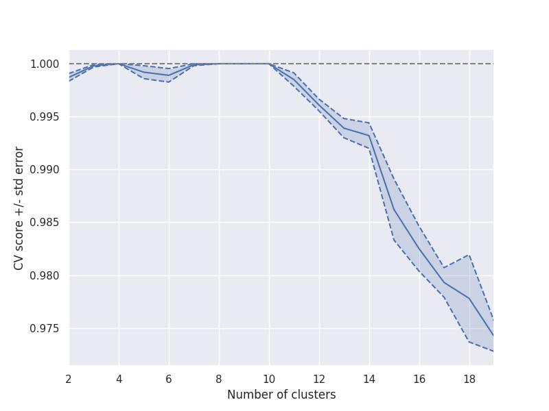
The results show an abrupt slope right after 10 clusters, which is commonly interpreted as a hint for maximum number of clusters.
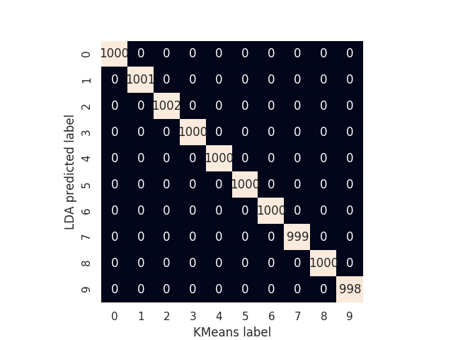
The accuracy and confusion matrix for the 10 clusters configuration are shown below.
# Code for plotting the confusion matrix taken from 'Python Data Science Handbook' by Jake VanderPlas

model.fit(X)
score = model.score(X)
print('Accuracy:',score)
kmeans_labels = model._predict_data[('clustering', 'predict')]
prediction = model.predict(X)

mat = confusion_matrix(y_true=kmeans_labels, y_pred=prediction)
sns.heatmap(mat.T, square=True, annot=True, fmt='d', cbar=False)
plt.xlabel('KMeans label')
plt.ylabel('LDA predicted label');
plt.show()
#%%
Out:
Accuracy: 1.0
Total running time of the script: ( 1 minutes 20.745 seconds)