Second example: GridSearchCV demonstration

This example shows how to use GridSearchCv with PipeGraph to effectively fit the best model across a number of hyperparameters. It is equivalent to use GridSearchCv with Pipeline. More complicated cases are shown in the following examples. In this second example we wanted to show how to fit a GridSearchCV in a yet simple scenario.

Steps of the PipeGraph:

• scaler: a preprocessing step using a MinMaxScaler object
• polynomial_features: a transformer step
• linear_model: the LinearRegression object we want to fit and use for predict.

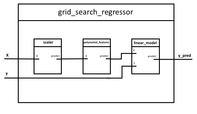
Figure 1. PipeGraph diagram showing the steps and their connections

Firstly, we import the necessary libraries and create some artificial data.

import numpy as np
from sklearn.preprocessing import MinMaxScaler
from sklearn.preprocessing import PolynomialFeatures
from sklearn.linear_model import LinearRegression
from sklearn.model_selection import GridSearchCV
from pipegraph.base import PipeGraph

import matplotlib.pyplot as plt

X = 2*np.random.rand(100,1)-1
y = 40 * X**5 + 3*X*2 +  3*X + 3*np.random.randn(100,1)

scaler = MinMaxScaler()
polynomial_features = PolynomialFeatures()
linear_model = LinearRegression()

Secondly, we define the steps and a param_grid dictionary as specified by GridSearchCV. In this case we just want to explore a few possibilities varying the degree of the polynomials and whether to use or not an intercept at the linear model.

steps = [('scaler', scaler),
         ('polynomial_features', polynomial_features),
         ('linear_model', linear_model)]

param_grid = {'polynomial_features__degree': range(1, 11),
              'linear_model__fit_intercept': [True, False]}

Now, we use PipeGraphRegressor as estimator for GridSearchCV and perform the fit and predict operations.

pgraph = PipeGraph(steps=steps)
grid_search_regressor = GridSearchCV(estimator=pgraph, param_grid=param_grid, refit=True)
grid_search_regressor.fit(X, y)
y_pred = grid_search_regressor.predict(X)

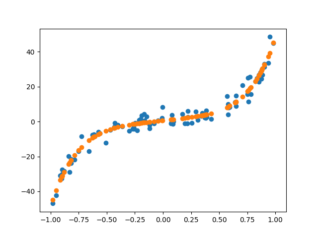
plt.scatter(X, y)
plt.scatter(X, y_pred)
plt.show()


coef = grid_search_regressor.best_estimator_.get_params()['linear_model'].coef_
degree = grid_search_regressor.best_estimator_.get_params()['polynomial_features'].degree

print('Information about the parameters of the best estimator: \n degree: {} \n coefficients: {} '.format(degree, coef))

Out:

Information about the parameters of the best estimator:
 degree: 5
 coefficients: [[  -44.9706866    363.27350854 -1281.17106722  2402.3058455
  -2319.31529496   925.19838541]]

This example showed how to use GridSearchCV with PipeGraphRegressor in a simple linear workflow. Next example provides detail on how to proceed with a non linear case.

Total running time of the script: ( 0 minutes 0.201 seconds)