Tenth Example: # Alternative solution to example number 9

We continue demonstrating several interesting features:

1. How the user can choose to encapsulate several blocks into a PipeGraph and use it as a single unit in another PipeGraph
2. How these components can be dynamically built on runtime depending on initialization parameters
3. How these components can be dynamically built on runtime depending on input signal values during fit
4. Using GridSearchCV to explore the best combination of hyperparameters

import numpy as np
import pandas as pd
import matplotlib.pyplot as plt
from sklearn.preprocessing import MinMaxScaler
from sklearn.mixture import GaussianMixture
from sklearn.linear_model import LinearRegression
from sklearn.model_selection import train_test_split

from pipegraph.base import ( PipeGraph,
                             ClassifierAndRegressorsBundle,
                             NeutralRegressor
                            )

X_first = pd.Series(np.random.rand(1000,))
y_first = pd.Series(4 * X_first + 0.5*np.random.randn(1000,))
X_second = pd.Series(np.random.rand(1000,) + 3)
y_second = pd.Series(-4 * X_second + 0.5*np.random.randn(1000,))
X_third = pd.Series(np.random.rand(1000,) + 6)
y_third = pd.Series(2 * X_third + 0.5*np.random.randn(1000,))

X = pd.concat([X_first, X_second, X_third], axis=0).to_frame()
y = pd.concat([y_first, y_second, y_third], axis=0).to_frame()

X_train, X_test, y_train, y_test = train_test_split(X, y)

Now we consider an alternative solution to example number 9. The previous solution showed the potential of being able to morph the graph during fitting. A simpler approach is considered in this example by reusing components and combining the classifier with the demultiplexed models:

import inspect
print(inspect.getsource(ClassifierAndRegressorsBundle))

Out:

class ClassifierAndRegressorsBundle(PipeGraph, RegressorMixin):
    def __init__(self, steps=[('classifier', GaussianMixture()), ('regressor', LinearRegression())]):
        self.steps = steps

    def fit(self, *pargs, **kwargs):
        classifier = self.named_steps.classifier
        regressor = self.named_steps.regressor
        number_of_clusters = query_number_of_clusters_from_classifier(classifier)
        multiple_regressors = RegressorsWithParametrizedNumberOfReplicas(number_of_replicas=number_of_clusters,
                                                                         regressor=regressor)

        steps = [('classifier', classifier), ('regressorsBundle', multiple_regressors)]
        connections = dict(classifier={'X': 'X'},
                           regressorsBundle={'X': 'X', 'y': 'y', 'selection': 'classifier'})
        self._adaptee = PipeGraph(steps=steps, fit_connections=connections)

        self._adaptee.fit(*pargs, **kwargs)
        return self

    def predict_dict(self, *pargs, **kwargs):
        return self._adaptee.predict_dict(*pargs, **kwargs)

Using this new component we can build a simplified PipeGraph:

scaler = MinMaxScaler()
classifier_and_models = ClassifierAndRegressorsBundle()
neutral_regressor = NeutralRegressor()

steps = [('scaler', scaler),
         ('bundle', classifier_and_models),
         ('neutral', neutral_regressor)]

connections = {'scaler': {'X': 'X'},
               'bundle': {'X': 'scaler', 'y': 'y'},
               'neutral': {'X': 'bundle', 'y': 'y'}}

pgraph = PipeGraph(steps=steps, fit_connections=connections)

Using GridSearchCV to find the best number of clusters and the best regressors

from sklearn.model_selection import GridSearchCV

param_grid = {'bundle__classifier__n_components': range(3,10)}
gs = GridSearchCV(estimator=pgraph, param_grid=param_grid, refit=True)
gs.fit(X_train, y_train)
y_pred = gs.predict(X_train)
plt.scatter(X_train, y_train)
plt.scatter(X_train, y_pred)
print("Score:" , gs.score(X_test, y_test))
print("bundle__classifier__n_components:", gs.best_estimator_.get_params()['bundle__classifier__n_components'])

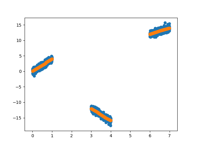
Out:

Score: 0.9978511505641998
bundle__classifier__n_components: 8

Total running time of the script: ( 0 minutes 2.655 seconds)