Third Example: Injecting varying sample_weight vectors to a linear regression model for GridSearchCV

This example illustrates a case in which a varying vector is injected to a linear regression model as sample_weight in order to evaluate them and obtain the sample_weight that generates the best results. Let’s imagine we have a sample_weight vector and different powers of the vector are needed to be evaluated. To perform such experiment, the following issues appear:

• The shape of the graph is not a linear sequence as those that can be implemented using Pipeline.
• More than two variables (typically: X and y) need to be accordingly split in order to perform the cross validation with GridSearchCV, in this case: X, y and sample_weight.
• The information provided to the sample_weight parameter of the LinearRegression step varies on the different scenarios explored by GridSearchCV. In a GridSearchCV with Pipeline, sample_weight can’t vary because it is treated as a fit_param instead of a variable.

Steps of the PipeGraph:

• selector: Featuring a ColumnSelector custom step. This is not a sklearn original object but a custom class that allows to split an array into columns. In this case, X augmented data is column-wise divided as specified in a mapping dictionary. We previously created an augmented X in which all data but y is concatenated and it will be used by GridSearchCV to make the cross validation splits. selector step de-concatenates such data.
• custom_power: Featuring a CustomPower custom class. A simple transformation of the input data that is powered to a specified power as indicated in param_grid.
• scaler: implements MinMaxScaler class
• polynomial_features: Contains a PolynomialFeatures object
• linear_model: Contains a LinearRegression model

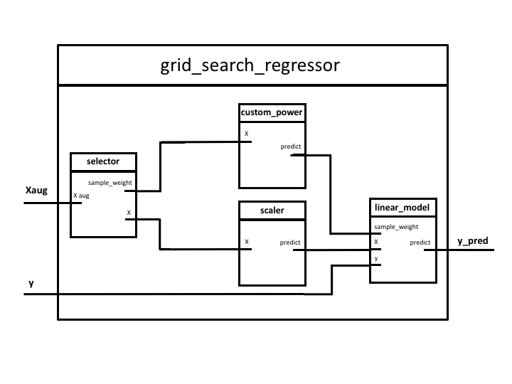
Figure 1. PipeGraph diagram showing the steps and their connections

import numpy as np
import pandas as pd
from sklearn.preprocessing import MinMaxScaler
from sklearn.preprocessing import PolynomialFeatures
from sklearn.linear_model import LinearRegression
from sklearn.model_selection import GridSearchCV
from pipegraph.base import PipeGraph, ColumnSelector, Reshape
from pipegraph.demo_blocks import CustomPower
import matplotlib.pyplot as plt

We create an augmented X in which all data but y is concatenated. In this case, we concatenate X and sample_weight vector.

X = pd.DataFrame(dict(X=np.array([   1,    2,    3,    4,    5,    6,    7,    8,    9,   10,   11]),
          sample_weight=np.array([0.01, 0.95, 0.10, 0.95, 0.95, 0.10, 0.10, 0.95, 0.95, 0.95, 0.01])))
y = np.array(                    [  10,    4,   20,   16,   25 , -60,   85,   64,   81,  100,  150])

Next we define the steps and we use PipeGraphRegressor as estimator for GridSearchCV.

scaler = MinMaxScaler()
polynomial_features = PolynomialFeatures()
linear_model = LinearRegression()
custom_power = CustomPower()
selector = ColumnSelector(mapping={'X': slice(0, 1),
                                   'sample_weight': slice(1,2)})

steps = [('selector', selector),
         ('custom_power', custom_power),
         ('scaler', scaler),
         ('polynomial_features', polynomial_features),
         ('linear_model', linear_model)]

pgraph = PipeGraph(steps=steps)

(pgraph.inject(sink='selector', sink_var='X', source='_External', source_var='X')
       .inject('custom_power', 'X', 'selector', 'sample_weight')
       .inject('scaler', 'X', 'selector', 'X')
       .inject('polynomial_features', 'X', 'scaler')
       .inject('linear_model', 'X',  'polynomial_features')
       .inject('linear_model', 'y', source_var='y')
       .inject('linear_model', 'sample_weight', 'custom_power'))

Then we define param_grid as expected by GridSearchCV exploring a few possibilities

of varying parameters.

param_grid = {'polynomial_features__degree': range(1, 3),
              'linear_model__fit_intercept': [True, False],
              'custom_power__power': [1, 5, 10, 20, 30]}



grid_search_regressor = GridSearchCV(estimator=pgraph, param_grid=param_grid, refit=True)
grid_search_regressor.fit(X, y)
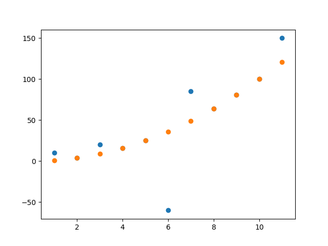
y_pred = grid_search_regressor.predict(X)

plt.scatter(X.loc[:,'X'], y)
plt.scatter(X.loc[:,'X'], y_pred)
plt.show()

power = grid_search_regressor.best_estimator_.get_params()['custom_power']
print('Power that obtains the best results in the linear model: \n {}'.format(power))

Out:

Power that obtains the best results in the linear model:
 CustomPower(power=20)

This example displayed a non linear workflow successfully implemented by PipeGraph, while at the same time showing a way to circumvent current limitations of standard GridSearchCV, in particular, the retriction on the number of input parameters. Next examples show more elaborated examples in increasing complexity order.

Total running time of the script: ( 0 minutes 0.519 seconds)